Fitting a Michaelis-Menten model to biochemical kinetics data
Biochem students will likely remember the mathematical beauty of enzyme kinetics models like the Michaelis-Menten model. In this short post, we'll take a look at how we can fit this kind of model to experimental data in Python using some staightforward optimization.
![]()
In [0]:
import numpy as np
from scipy.optimize import minimize
import matplotlib.pyplot as plt
Let's assume we are measuring reaction rate $v$ as a function of substrate concentration $[S]$ under a simple Michaelis-Menten model:
$$ v = \frac{V_{max}[S]}{K_M + [S]} $$In [0]:
def v(s, v_max, k_m):
    return (v_max * s) / (k_m + s)
We perform experiments to collect some data points $D$ where the $i$th row of $D$ is $d_i = ([S]_i, v_i)$.
In [0]:
data = np.array([[3.6, 1.8, 0.9, 0.45, 0.225, 0.1125, 3.6, 1.8, 0.9, 0.45, 0.225, 0.1125, 3.6, 1.8, 0.9, 0.45, 0.225, 0.1125, 0],
                 [0.004407692, 0.004192308, 0.003553846, 0.002576923, 0.001661538, 0.001064286, 0.004835714, 0.004671429, 0.0039, 0.002857143, 0.00175, 0.001057143, 0.004907143, 0.004521429, 0.00375, 0.002764286, 0.001857143, 0.001121429, 0]]).T

v_real = data[:, 1]
s_real = data[:, 0]
data
Out[0]:
We can then fit the two parameters $V_{max}$ and $K_M$ using this data.
We first specify a least squares loss function:
In [0]:
def loss(theta):
    v_max, k_m = theta
    v_pred = v(s_real, v_max, k_m)
    return np.sum((v_real - v_pred)**2)
And then optimize it:
In [0]:
res = minimize(loss, [1, 1])
res.x
Out[0]:
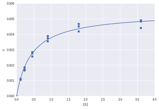
Finally, we can plot the fitted model over the real data points:
In [0]:
plt.scatter(s_real, v_real)
s_plot = np.linspace(0, 4, 100)
plt.plot(s_plot, v(s_plot, res.x[0], res.x[1]))
plt.xlim([0, 4])
plt.ylim([0, 0.006])
plt.xlabel('$[S]$')
plt.ylabel('$v$')
plt.show()

Comments
Comments powered by Disqus