Linear regression in Python (UPenn ENM 375 guest lecture)

I was recently invited to give a guest lecture in the course ENM 375 Biological Data Science I - Fundamentals of Biostatistics at the University of Pennsylvania on the topic of linear regression in Python. As part of my lecture, I walked through this notebook. It might serve as a useful reference, covering everything from simulation and fitting to a wide variety of diagnostics. The walkthrough includes explanations of how to do everything in vanilla numpy/scipy, scikit-learn, and statsmodels. As a bonus, there's even a section on logistic regression at the end.

Read on for more!

1 Simulating data from linear models¶

Simulate $N$ data points from the linear model

$$y = X\beta + \epsilon \;,\quad \epsilon \sim \mathcal{N}(0, \sigma)$$

We will make the first column of $X$ all 1's so that the first element of $\beta$ represents an intercept. For example:

\begin{align} y &= X\beta + \epsilon \\ \begin{bmatrix} y_1 \\ y_2 \\ \vdots \end{bmatrix} &= \begin{bmatrix} 1 & x_1 \\ 1 & x_2 \\ \vdots & \vdots \end{bmatrix} \begin{bmatrix} \beta_0 \\ \beta_1 \end{bmatrix} + \begin{bmatrix} \epsilon_1 \\ \epsilon_2 \\ \vdots \end{bmatrix} \\ y_i &= \beta_0 + \beta_1 x_i + \epsilon_i, \quad i=1,2,\ldots, N \end{align}

2 Ordinary least squares parameter fitting¶

2.1 Normal equations¶

We want to find an estimate $\hat{\beta}$ given some observations $y, X$ such that we make $X\hat{\beta}$ as close as possible to $y$ in terms of squared differences:

\begin{align} \hat{\beta} &= \mathrm{arg} \min_\beta ||y - X\beta ||^2 \\ &= \mathrm{arg} \min_\beta \; (y - X\beta)^T(y - X\beta) \\ &= \mathrm{arg} \min_\beta \; y^Ty-(X\beta)^T y - y^T(X\beta)+(X\beta)^T(X\beta) \\ &= \mathrm{arg} \min_\beta \; y^Ty- 2\beta^T X^T y +\beta^T X^T X\beta \end{align}

Taking the derivative of this expression and looking for critical points, we find

\begin{align} \frac{d}{d\hat{\beta}}\left(y^Ty- 2\hat{\beta}^T X^T y +\hat{\beta}^T X^T X\hat{\beta}\right) &= 0 \\ -2 X^T y +2 X^T X\hat{\beta} &= 0 \\ 2 X^T X\hat{\beta} &= 2 X^T y \\ X^T X\hat{\beta} &= X^T y \\ (X^T X)^{-1} X^T X\hat{\beta} &= (X^T X)^{-1} X^T y \\ \hat{\beta} &= (X^T X)^{-1} X^T y \end{align}

2.2 Covariance equation¶

We can also estimate the slope $\hat{\beta}_1$ as $$\hat{\beta}_1 = \frac{\mathrm{Cov}(x_{:, 1}, y)}{\mathrm{Var}(x_{:, 1})}$$

2.3 Rescaled correlation coefficient¶

We can also estimate the slope $\hat{\beta}_1$ using the correlation coefficient $r_{xy}$ and the sample standard deviations of $x$ and $y$, respectively

$$\hat{\beta}_1 = r_{xy}\frac{s_y}{s_x}$$

This basically works because the Pearson correlation is the slope of the least squares line through the data points after they've been centered and scaled.

$$z_y = \frac{y - \bar{y}}{s_y}, \quad z_x = \frac{x - \bar{x}}{s_x}$$

Centering doesn't change the slope, but we can undo the scaling (division/multiplication by standard deviation).

2.4 scikit-learn¶

sklearn.linear_model.LinearRegression will automatically add a column of 1's to $X$ and store the coefficient for that column (the intercept) at model.intercept_. Since we already have 1's in our $X$ matrix, we can pass fit_intercept=False to avoid this.

We can also pass just the $X_{:, 1}$ values, but note that we have to make sure to pass $X$ as a matrix whose rows correspond to observations and whose columns correspond to features, so we expand the 1-dimensional x[:, 1] back to a column vector x[:, 1][:, None].

2.5 statsmodels¶

statsmodels uses an R-like "formula API" which allows you to specify which variables (on the right of the ~) you want to use to fit what other variable (on the left of the ~) where the variables are column names in a pandas DataFrame which you might load from a table of data on disk.

statsmodels computes a bunch of useful information about the regression, some of which we will dig into below.

3 Residuals and diagnostics¶

In the context of prediction (or projection), the values in $y$ predicted by our model (or projected onto the subspace spanned by the columns of $X$) are

$$\hat{y} = X\hat{\beta}$$

The "residuals" of the fit are the difference between this predicted $\hat{y} = X\hat{\beta}$ and the original $y$ values:

$$r = X\hat{\beta} - y$$

3.1 Normality¶

We can look at the distribution of the residuals using either a histogram or a QQ plot, and test it for normality. There are many tests for normality, but one common one is the "omnibus" test mentioned in the statsmodels summary table and implemented in scipy.stats.normaltest(). This tests the null hypothesis that the residuals are in fact normally distributed.

3.2 Linearity¶

If the relationship between the variables really is linear, we expect the residuals to be scattered around zero (both above and below) across the x-axis. One way to test this quantitatively is with the Harvey-Collier test (tests the null hypothesis that the relationship between the variables is linear):

3.3 Homoscedasticity¶

To be more specific, we expect to see that the residuals are scattered around zero with a variance that doesn't depend on $X$ (or anything else really). One way to test this quantitatively is with the Breusch-Pagan test (tests the null hypothesis that the data are homoscedastic).

3.4 Independence¶

For ordered data, we can plot a scatterplot of the residuals versus observation number and/or the autocorrelation of the residuals. Even if data are nominally unordered, oftentimes the order of rows in a data table can reveal something about the time periods in which data were collected, etc. The Durbin-Watson test is used by statsmodels to attempt to quantify the degree of correlations in the residuals - it doesn't come with an automatically computed p-value, however, and instead is simply a number between 0 and 4 which should be close to 2 if there is no sequential correlation in the residuals.

3.5 First-order conditions¶

If we picked our estimate for the slope $\hat{\beta}_1$ correctly, it should "regress out" all the correlation between $X$ and $y$ such that nothing is left in the residuals.

4 Inference and significance¶

So far we have covered how to estimate and diagnose the point estimates of the parameters $\hat{\beta}$. Now we will discuss how to quantify the uncertainty in the model (and thereby assess the significance of the relationships quantified by $\hat{\beta}$).

4.1 Standard error of the model¶

This process starts with estimating the variance of the error term $\epsilon$, which we called $\sigma^2$ above. We can form an estimate $\hat{\sigma}^2$ of this variance from the residuals:

$$\hat{\sigma}^2 = \frac{r^T r}{n - p}$$

where $n-p$ represents the degrees of freedom in the regression (the number of observations $n$ minus the number of coefficients we fitted $p$).

This quantity is computed by statsmodels and saved as results.scale.

4.2 Standard errors of the coefficients¶

Our estimates for the variances of our estimates of the coefficients $\hat{\beta}$ are then

$$\hat{\mathrm{Var}}[\hat{\beta} \mid X] = \hat{\sigma}_\beta^2 = \hat{\sigma}^2 (X^T X)^{-1}$$

statsmodels prints the square root of the estimated variances for each coefficient in $\hat{\beta}$ in the summary table, calling them "std err'', and stores them in results.bse.

We can use these standard errors to both

1. test to see if the coefficients are significant (using a t-test), and
2. compute confidence intervals for the coefficients.

4.3 Significance of the coefficients¶

To do (1) we first compute the t-statistic against the null hypothesis that the coefficient is zero (stored by statsmodels in results.tvalues):

We can then compute two-tailed p-values (since we plan to reject the null hypothesis of $\beta = 0$ regardless of the sign of the coefficient) by comparing the t-statistics against a t-distribution with $n - p$ degrees of freedom (stored by statsmodels in results.pvalues):

4.4 Confidence intervals for the coefficients¶

To do (2), we find the appropriate percentiles of t-distribution we just used above for calling the p-values, scale them by $\hat{\sigma}_\beta$, and shift them by $\hat{\beta}_i$:

We can also perform this shifting and scaling using the loc and scale kwargs in scipy.stats:

statsmodels also computes 95% confidence intervals for the coefficients and prints them in the table under the heading "[0.025 0.975]". You can also compute any confidence intervals you like by calling results.conf_int():

5 Multiple linear regression¶

In general each observed data point may have multiple features (or things we measure about it). These correspond to new rows of $X$ and new elements in $\beta$ in the matrix equation for our linear model:

\begin{align} y &= X\beta + \epsilon \\ \begin{bmatrix} y_1 \\ y_2 \\ \vdots \end{bmatrix} &= \begin{bmatrix} 1 & x_{11} & x_{12} & x_{13} & \cdots \\ 1 & x_{21} & x_{22} & x_{23} & \cdots\\ \vdots & \vdots & \vdots & \vdots & \ddots \end{bmatrix} \begin{bmatrix} \beta_0 \\ \beta_1 \\ \beta_2 \\ \beta_3 \\ \vdots \end{bmatrix} + \begin{bmatrix} \epsilon_1 \\ \epsilon_2 \\ \vdots \end{bmatrix} \end{align}

5.1 Simulation¶

Our simulation code still looks very similar:

5.2 Normal equations¶

and the same exact normal equations we used above will still work:

5.3 Multiple linear regression as multiple single variable linear regressions¶

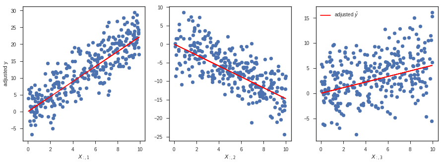
Plotting (and thinking) in higher dimensions is tricky, but one convenient way to think about multiple linear regression is that it estimates $\hat{\beta}_i$ by performing a simple linear regression between $X_{:, i}$ and a version of $y$ that has been adjusted for all the other columns of $X$.

In the code block below, y23 represents a version of $y$ that has been adjusted for the 2nd and 3rd columns of $X$. What I mean here by "adjusted" is simply that the linear dependence on those columns has been "regressed out" (i.e., subtracted from) $y$. To do this in code, I just take $y$ and subtract the $\hat{y}$ I would get if I used only the 2nd and 3rd columns of $X$ to predict $\hat{y}$. Mathematically:

$$y_{23} = y - \hat{y}_{23}$$$$\hat{y}_{23} = X_{:,23} \times \hat{\beta}_{23}$$

where $X_{:,23}$ represents all the rows (:) but only the 2nd and 3rd columns of $X$, and $\hat{\beta}_{23}$ represents the corresponding entries of $\hat{\beta}$.

Note that in this case I'm not regressing out the intercept $\hat{\beta}_0$ - this is a bit of an oversimplification. In this specific simulation, we set the true value of the intercept $\beta_0$ to 0, but this would not be true in general. Moreover, our estimate of $\hat{\beta}_0$ is nonzero. To be truly correct here, we could either add our estimated intercept $\hat{\beta}_0$ to the red line (e.g., ax1.plot(x[:, [0, 1]], x[:, [0, 1]] * beta_hat[[0, 1]], ...)), or we could ensure that the adjusted $y$ values are also adjusted for the intercept (e.g., replace y23 with y023 = y - x[:, [0, 2, 3]] @ beta_hat[[0, 2, 3]]). In this specific case, it wouldn't change the appearance of the plot by much because $\hat{\beta}_0$ is relatively small.

All of the diagnostics discussed above can be applied to the residuals just as before.

5.4 scikit-learn¶

sklearn.linear_model.LinearRegression works just as before:

5.5 statsmodels¶

statsmodels also works just as before:

6 Logistic regression¶

6.1 The logistic regression model¶

The logistic regression model is

$$y_i \sim \mathrm{Bernoulli}(p_i), \quad \ln \frac{p_i}{1-p_i} = X_{i,:}^T\beta $$

were $y_i$ is a boolean variable representing the $i$th observation, $\ln\frac{p_i}{1-p_i}$ represents the log odds for the $i$th observation being a success, $X_{i,:}$ represents all the features we observe for the $i$th observation, and $\beta$ is a vector of weights.

The function

$$f(p) = \ln \frac{p}{1-p}$$

is called the logit function. Its inverse function is

$$f^{-1}(x) = \frac{1}{1+\exp(-x)}$$

and is called the logistic function (but is called scipy.special.expit() in scipy).

6.2 Simulating from a logistic model¶

Our simulation looks similar to the linear regression simulation above, except for the following important differences:

1. There is no error term $\epsilon$. In the logistic regression model, randomness comes directly from the Bernoulli distribution.
2. We use the logistic function (scipy.special.expit()) to "link" the linear combination of our predictors $X$ weighed by our weights $\beta$ to the Bernoulli distribution parameter $p$. Don't think too hard about it now, but this is the basic principle underlying generalized linear models (GLMs). Conveniently, the range of the logistic function is $(0, 1)$, which means that any number it returns will be a valid Bernoulli parameter $p$.

We can visualize our simulated data on a scatterplot as before, but this time the $y$-values can take on only two values (1 and 0, the support of the Bernoulli distribution). We can visualize the relationship between $x$ and the probability that a point at that $x$ value will result in a successful Bernoulli trial as a function $p(x)$ (a logistic function parameterized by $\beta$), which is the red curve in the plot below.

6.3 Fitting logistic regression parameters¶

To draw the red curve above, we computed $p = \mathrm{expit}(X^T\beta)$ using the true value of $\beta$. Our goal when fitting the logistic regression model will be to compute estimates $\hat{\beta}$ directly from the observed data ($X$ and $y$) and thereby obtain an estimated probability curve $\hat{p}(x)=\mathrm{expit}(x^T\hat{\beta})$.

Unlike linear regression, there is no closed-form solution for estimating the logistic regression parameters $\beta$, so we will do this using iterative methods (usually some variation on Newton's method).

6.3.1 scikit-learn¶

6.3.2 statsmodels¶